Any Excel user who considers themselves a “power user” cannot make such a statement with a straight face without knowing how to use VLOOKUP functions.

Of all of the ways to retrieve information, the VLOOKUP function is without debate the most popular means of looking up and returning information from an Excel list.  It’s not the most versatile lookup tool Excel has to offer (there are a few situations where it can’t get the job done), but for most scenarios, it works quite well.

Before we see how to improve the performance of this popular function, we need to understand a few key behavioral characteristics, both good and bad.

(Feel free to skip to “The New (and Possibly Worse) Problem” section below if you are already familiar with how VLOOKUP match logic works.)

Approximate Match vs. Exact Match Searches

Excel can be instructed to retrieve data from a list in one of two modes:

• Return the requested item or return an error if the requested item is not found (also known as an exact match)
• Return the requested item or return the closest item in the list to the requested item without going over (also known as an approximate match)

Let’s look at an example.

Exact Match

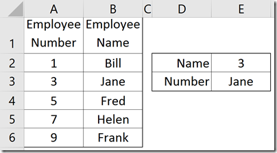
If we wanted to search for a known employee number and discover who is assigned to that number, we could construct a structure like the following:

Cell E2 is where the user types in an employee number

Cell E3 contains =VLOOKUP(E2,A2:B6,2)

The above VLOOKUP function is broken down with the following logic:

• E2 defines the cell containing the information we know (employee number)
• A2:B6 defines the table containing the desired information
• 2 defines the column position (counting left to right) that we wish to return information from

If we feed cell E2 a number, like “3”, the VLOOKUP function will scan the first (leftmost) column of the table defined by A2:B6 and locate the requested number.  When that number is found, the VLOOKUP with return the information located in the second column (“Jane”, defined by the 2.)

The Problem

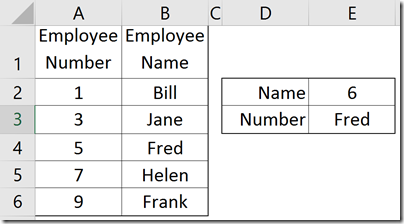
A problem occurs when a user defines a value to search for that does not exist in the list.

Clearly, employee number “6” does not exist in the list, but the VLOOKUP function still returns an answer of “Fred”.  The reason this happens is that by default, if the VLOOKUP function fails to located the requested item, it will return data related to the closest item in the search column without going over.  In other words, “I couldn’t find the number ‘6’ in the first column, so I’ll use ‘5’ instead since it’s the closest number in the list to ‘6’ without going over ‘6’.”

For most of us, this presents a REAL problem, because if we didn’t know any better, we would just trust the returned result of “Fred” and move along our merry way.

The Solution

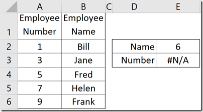
By adding an additional parameter to our VLOOKUP function, we can instruct VLOOKUP to return an error if the item is not found instead of this “closest without going over” business.  The new formula would look like the following:

Cell E3 contains =VLOOKUP(E2,A2:B6,2,FALSE)

The “FALSE” variable instructs VLOOKUP to only return data if the requested value is located in the first column; otherwise, an error message will be displayed.

Making the Answer More User-Friendly

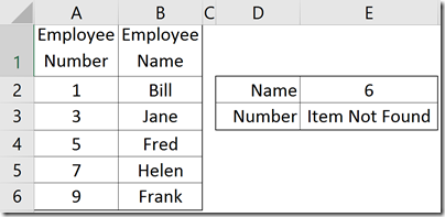
Because most users will not understand what is meant by the “#N/A” error message, we can customize the error message by nesting the original VLOOKUP function inside of an IFERROR function.

=IFERROR(VLOOKUP(E2,A2:B6,2,FALSE),”Item Not Found”)

This would result in the following improved response:

The New (and Possibly Worse) Problem

In terms of performance, comparing the performance of an approximate match against an exact match search is like racing a tortoise vs. the hare.  Approximate match searches are REALLY fast, whereas exact match searches are really slow.  The reason for this is the strategy employed by the VLOOKUP.

When executing an approximate match, VLOOKUP utilizes what is known as a Binary Search.

IMPORTANT NOTE: Binary Searches require the list be sorted in ascending order by the left-most column; the column being searched.

In essence, a binary search starts in the middle of the list and says “Is this it?”  If it is, you win.  If it is not, it checks to see if the item it landed on is either higher or lower than what it was looking for.  If the discovered value is HIGHER than what it is looking for, everything after that point is ignored and it now examines what remains (the first half of the list.)  If the discovered value is LOWER than what it is looking for, everything before that point is ignored and it now examines what remains (the last half of the list.)

With the remaining half of the original list, VLOOKUP selects a record halfway into the list and performs the same “is it higher or is it lower” strategy as before.  VLOOKUP will repeat this process until it locates the requested item or runs out of things to cut in half, at which point it simply returns the final remaining item.

What is so great about this strategy is that regardless of list length, the target item can be located within relatively few steps.  For example, a list of 1,000,000 records can, in a worst-case scenario, locate the requested item in only 20 steps.

When executing an exact match, VLOOKUP utilizes what is known as a Linear Search.

A linear search starts with the first record and examines each record, one at a time, in order and stops when it locates the requested item or runs out of records to examine, at which point it will return an error message of #N/A.  Using the same 1,000,000 record example, the worst-case scenario is 1,000,000 steps.  On average, searches will take 500,000 steps.  Compared to 20 steps, that is quite a difference.

Making Things Even WORSE

Because VLOOKUP is considered a “volatile function”, if you have hundreds or thousands of VLOOKUP functions in a sheet and you change the contents of any cell, ALL of the VLOOKUP functions must recalculate.  That means potentially BILLIONS of unnecessary recalculations which translates into a poorly performing worksheet.

The Supercharged Solution

There is a very clever way to leverage the speed of the approximate match strategy with the precision of the exact match strategy, and that is to PERFORM THE VLOOKUP TWICE!  I realize this sounds completely insane, but it is actually quite ingenious.

If we employ the assistance of an IF function, we can execute what is essentially a pre-test search on the data to see if the value exists.

=IF(VLOOKUP(E2,A2:B6,1)<>E2,”Item Not Found”)

By using a binary search, we can determine in just a few steps if the item exists.  This is done by comparing the return result (notice that the VLOOKUP is returning an item from the FIRST column of the list) with the originally searched for value to see if they match.  If they match, we know the item is in the list.  If they do not match, then we know the item is NOT in the list and we can issue a message of our choosing.  Technically, since we are only concerned with the first column we could modify the VLOOKUP as follows:

=IF(VLOOKUP(E2,A2:A6,1)<>E2,”Item Not Found”)

This modification, although subtle, only scans one column instead of an entire array of columns as was done originally.

This formula gets us close, but is not quite complete.  The above formula only executes the pre-test search and returns a message if the item is not located; it does not return any related data if the requested item is located.  Enter the final solution:

=IF(VLOOKUP(E2,A2:A6,1)<>E2,”Item Not Found”,(VLOOKUP(E2,A2:B6,2))

As you can see, if the pre-test search fails, we issue the message; but if the pre-test passes, we execute the VLOOKUP a second time, safe in the knowledge that we will discover the requested item in the list and can then return some related information.

CONCLUSION

Even if we have to execute TWO VLOOKUP functions on a list of 1,000,000 records, the most steps this will take is 40 steps.  Compared to an average of 500,000 steps for a single VLOOKUP using exact match logic, the choice is clear.

BONUS NOTES

• If you wish to sort your list by some other column (i.e. “Employee Name”), you CANNOT use these strategies; you will be forced to use the exact match logic and just take the performance hit.
• An alternative to the final formula, if you would rather identify existing records as opposed to missing records, would be to rewrite the formula as follows:

=IF(VLOOKUP(E2,A2:A6,1)=E2,(VLOOKUP(E2,A2:B6,2), ”Item Not Found”)

• Since the binary search will only result in 20 or so steps in the longest Excel table, you can simply examine the entire search column regardless of table length (notice the lack of row number declarations):

=IF(VLOOKUP(E2,A:A,1)=E2,(VLOOKUP(E2,A:B,2), ”Item Not Found”)