Anyone who has ever used Excel and needed to query a table for information has no doubt used a VLOOKUP function. VLOOKUP is one of the most widely used functions in all of Excel. But even the most popular things in life are not without their shortcomings.
The single most vexing problem for VLOOKUP users is ensuring that the column of known values (known as the “key column”) must reside to the LEFT of any column whose value is to be returned. Just like looking at a menu in a restaurant, you scan down the left side of the list for the item name and then look to the right for the price.
But what if your data is structured in such a way that the column you with to return data from is to the LEFT of the column being searched?
The most common approach to solving this problem is to restructure the data so that the return column is positioned to the RIGHT of the key column. This restructuring of the data not only takes time to perform, it also provides a prime opportunity to introduce errors into your data. There is also the possibility that you are not able to restructure the data for business or workflow reasons.
CHOOSE to the Rescue!
Excel has an interesting, yet often overlooked function, called CHOOSE. The CHOOSE function is extremely simple to use. The basic purpose of CHOOSE is to return an item in a list from a position you specify. If that sounds like VLOOKUP or INDEX, the difference is that CHOOSE has no physical list on the spreadsheet to work from. All the list items are contained within the function itself.
Let’s look at a simple example.
We want the user to enter a number between 1 and 4 in cell “C1”. In return, a city name will be displayed in cell “C3”. As you can see from the illustration below, if the user enters a “3” the returned city name is “Denver”.
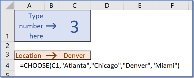
Instead of having a list like the following…
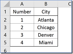
…we can contain the entirety of the logic within the CHOOSE function.
=CHOOSE(C1,”Atlanta”,”Chicago”,”Denver”,”Miami”)
The CHOOSE function simply returns an item in its list from the position specified in the first variable (in this case, “C1”.) If “C1” says “3”, the returned city name is “Denver”.
Normally, we would leave the first variable pointing to an input cell so the user could define the number. What if we hard-coded the first variable?
=CHOOSE(3,”Atlanta”,”Chicago”,”Denver”,”Miami”)
The above example would still return the city “Denver” but the user would have no way to change the number to return a different city. On its face, this seems like a step backwards in functionality. This is where the elegance kicks in.
Building a Virtual Table
Let’s suppose we have a table where the key column is to the RIGHT of the return data.
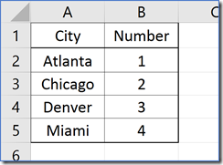
VLOOKUP has no ability to scan column “B” and return data from column “A”. Since we are prohibited to rearrange the data, let’s build a new table virtually in memory with the CHOOSE function.
=CHOOSE({1,2},B2:B5,A2:A5)
By replacing the first variable with {1,2} we are saying, “Let’s get BOTH options from the list and stick them side-by-side”, thereby creating a new virtual table in computer memory.
The {1,2} allows us to create an array of data {1,”Atlanta”;2,”Chicago”;3,”Denver”;4,”Miami”} (Side note: if you are not familiar with array syntax, commas separate items on the same row while semi-colons separate rows. Also, arrays must be enclosed in curly braces.)
With this new list in computer memory, we can use it as the source list to be queried by a VLOOKUP function.
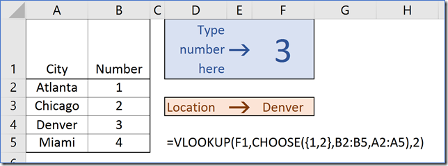
=VLOOKUP(F1,CHOOSE({1,2},B2:B5,A2:A5),2)
In a nutshell, the CHOOSE function builds a virtual table where we rearrange the original tables columns in any order we wish. This new virtual table becomes the source table for the VLOOKUP function.
Caveat: Because you are building another table in memory, if the original table is large (for the sake of argument, let’s say 500K records) this could impact spreadsheet performance.
BONUS IDEA:
We can use this strategy to take regular, normally structured tables that contain large numbers of unneeded columns and reduce it to a virtual table with only the needed columns.

The above table with 15 columns (and 200 rows) of data can be reduced to a virtual table consisting of two columns (below)
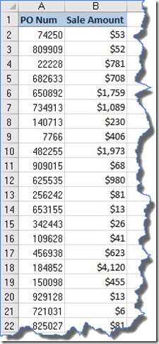
To lookup the Sale Amount in the original table, the formula would be as follows (“XX” is the input cell):
=VLOOKUP(XX,A2:O200,15,0)
The updated formula for the virtual table would be as follows:
=VLOOKUP(XX,CHOOSE({1,2},A2:A200,O2:O200),2,0)
This may appear to be making things more complicated, but in reality, by simply changing the “O2:O200” with another column letter, we can query something completely different without having to revise column index positions in the VLOOKUP; everything is returned from “Column 2”.
