Locating a specific item in a table based on two separate criteria can be a challenging task, even for the most ardent Excel user. Take the following table, for example:

Suppose you wish to locate the sales for the Southern region in the month of March. You could try to write a sophisticated VLOOKUP with a nested MATCH function like the one below.
=VLOOKUP(“Southern”,A1:G6,MATCH(“Mar”,A1:G1,0),FALSE)
or
you could write something more elegant like
=D:D 4:4
“WHAT?!?!?!?!”, you’re undoubtedly saying to yourself. “How can it be that simple?” The trick to it all is the use of the INTERSECTION OPERATOR.
By using a “space” between two references, as in this case, the column that holds Mar and the row that holds Southern, you are asking Excel to return the information in the cell where those two ranges cross.
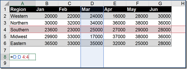
It’s just like asking Google Maps, “What’s at the intersection of 4th Avenue and Main Street?”, and it came back saying “Starbuck’s”. In this case, we are asking Excel, “What is at the intersection of Column D and Row 4?” The answer is 25000.
Thing Get Even Better with Named Ranges
If we were to create named ranges out of the data, we could then use the nice user-friendly names instead of the native (and when I say “native” I mean “ugly”) cell references.
Step 1: Create the Named Ranges FAST
Select the data and then click on the FORMULAS tab and select “Create from Selection” located in the DEFINED NAMES group.

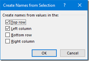
Make sure that “Top row” and “Left column” are selected and click OK.
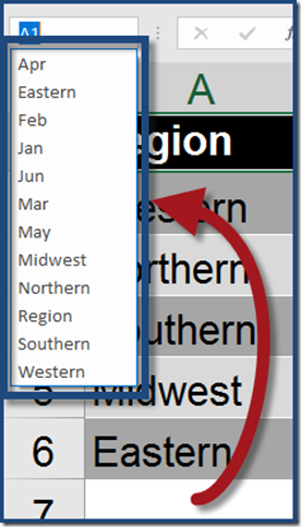
You will now have a nice list of named ranges corresponding to the row and column headings in the data.
Step 2: Use the range names in lieu of the native cell references
=Southern Mar
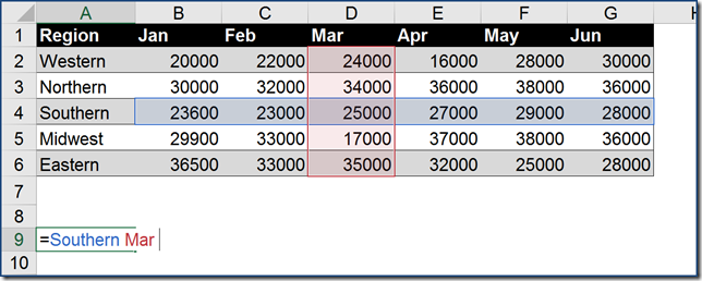
And there you have it; the answer to “What is at the intersection of Southern and Mar?” 25000.
The Cherry on Top…
To make things even better, let’s give the user the ability to select their region and month from a dropdown list so that the query can be dynamic.
Step 1: Create two Data Validation lists from the original table
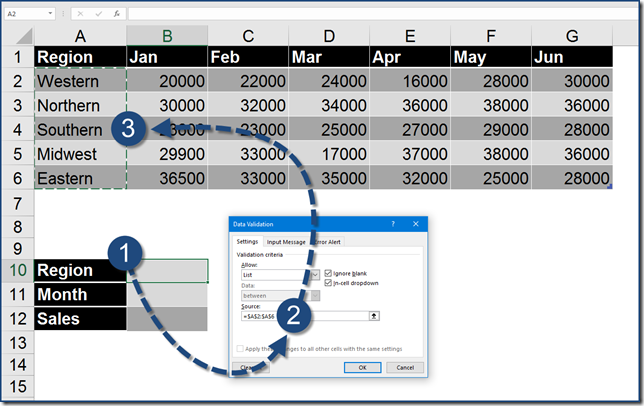
Create a data validation dropdown list using the region names. If you are not familiar with creating Data Validation dropdown lists, click here.
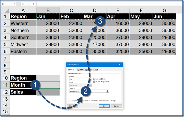
Repeat the process to create a data validation list using the month names
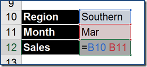
Step 2: Create a formula that takes values selected by the user for Region (B10) and Month (B11) and uses them to find the intersection of those ranges.
=B10 B11
Oh, No! What happened? It appears to have failed.
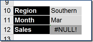
The reason this failed to produce the desired result is because your formula is attempting to find a value at the intersection of B10 and B11. These two cells do not intersect with one another. What we really need is to use the selections contained within B10 and B11, not the cell addresses themselves.
INDIRECT to the Rescue
The Excel INDIRECT function is one of those ninja-level functions that most users have never heard of. INDIRECT basically says, “Use what’s inside of this cell as the reference, not the cell address itself.” It basically substitutes the cell address with the contents of the cell.
=INDIRECT(B10) INDIRECT(B11)

This will now rewrite the formula from this
=INDIRECT(B10) INDIRECT(B11)
to this
=INDIRECT(“Southern”) INDIRECT(“Mar”)
which in turn produces the desired result.
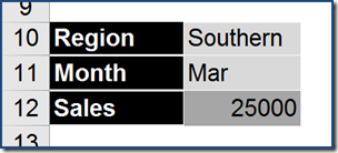
The user is now able to select any region and any month form the two dropdown menus and the Sales field will display the proper answer.
