An ordinal indicator is a character, or group of characters, that follows a number denoting that it is an ordinal number, as opposed to a cardinal number.
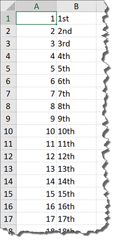
For English speaking countries, this corresponds to the suffixes -st, -nd, -rd, -th in written ordinals (represented either on the line 1st, 2nd, 3rd, 4th or as superscript, 1st, 2nd, 3rd, 4th).
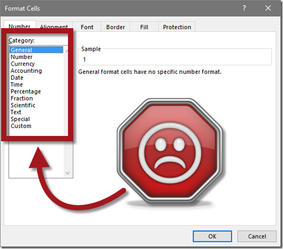
The unfortunate issue with Excel number formatting is that there is no way to apply ordinal suffixes to a list of numbers.

Luckily, with the help of a few Excel functions working as a team we can produce the desired list of numbers. The functions required to pull off this feat of formulaic legerdemain are:
- IF
- AND
- ABS
- IFERROR
- CHOOSE
- MOD
- CONCATENATE (&)
(When was the last time you used SEVEN functions in a single formula? This is truly the stuff of ninjas.)
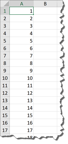
Suppose we have a list of numbers in Column A in our Excel spreadsheet.

We will now enter the formula shown below into cell B1 and then Fill Down Column B to the same row as the last number in the list.
=A1&IF(AND(MOD(ABS(A1),100)>10,MOD(ABS(A1),100)<14),”th”,IFERROR(CHOOSE(MOD(ABS(A1),10)+1,”th”,”st”,”nd”,”rd”),”th”))
If that is not enough to make you run screaming for the nearest fire exit, I don’t know what will. It’s really not that bad if you break it down into its components. Let’s see if we can make some sense of this behemoth.
NOTE: This formula could actually be much simpler if it weren’t for just a handful of pesky troublemaker numbers. I’m speaking of the numbers 11, 12, and 13. Unlike all of the other uses of the numbers 1, 2, and 3 when they are used in the 1’s position, they end in “st”, “nd”, and “rd” respectively. It’s only when we use them as an 11, 12, or 13 (what we will refer to as the “teens block”) that we have to use the suffix “th”. Anyplace else where we would see something like “131st, 132nd, and 133rd”, we have to write it as “11th, 12th, and 13th” when in the “teens block” of numbers.
Before you lose your collective minds, screaming at the display, “Doesn’t this chump know you can to this in 5 seconds with a Fill Series operation?” Yes… I do. This solution is for when you want to present a number with its ordinal suffix, such as in a dashboard report.
Step 1: Convert all numbers to positive numbers
Since we will have difficulty dealing with negative numbers, we must first convert any negative numbers to positive numbers. We will use the ABS (Absolute) function ensuring all examined numbers are positive numbers. (Don’t worry; if the original number is negative, it will return to negative in the last step, the CONCATENATE step.)
=A1&IF(AND(MOD(ABS(A1),100)>10,MOD(ABS(A1),100)<14),”th”,IFERROR(CHOOSE(MOD(ABS(A1),10)+1,”th”,”st”,”nd”,”rd”),”th”))
Step 2: Check to see if we are in the “teens block”
The MOD function will assist with this determination. By dividing the number by 100 and keeping only the remainder, we can pass the remainder to the AND function (Step 3) who will determine if the number falls within the “teens block”. If it helps, imagine the MOD/100 function stripping off the 100’s place number and leaving us with a two-digit number.
=A1&IF(AND(MOD(ABS(A1),100)>10,MOD(ABS(A1),100)<14),”th”,IFERROR(CHOOSE(MOD(ABS(A1),10)+1,”th”,”st”,”nd”,”rd”),”th”))
Step 3: Check to see if the number is 11, 12, or 13
In order to see if the number is greater than 10 and less than 14 we have to use an AND function so we can check two conditions:
- The first question will test to see if the number is greater than 10
- The second question will test to see if the number is less than 14
=A1&IF(AND(MOD(ABS(A1),100)>10,MOD(ABS(A1),100)<14),”th”,IFERROR(CHOOSE(MOD(ABS(A1),10)+1,”th”,”st”,”nd”,”rd”),”th”))
If both of these AND statements result in TRUE responses, the IF function will select “th” from the Value if True portion of the IF function.
=A1&IF(AND(MOD(ABS(A1),100)>10,MOD(ABS(A1),100)<14),”th”,IFERROR(CHOOSE(MOD(ABS(A1),10)+1,”th”,”st”,”nd”,”rd”),”th”))
Of course, if one, the other, or both AND statements result in FALSE responses, the IF function will select its Value if False option.
=A1&IF(AND(MOD(ABS(A1),100)>10,MOD(ABS(A1),100)<14),“th”,IFERROR(CHOOSE(MOD(ABS(A1),10)+1,”th”,”st”,”nd”,”rd”),”th”))
*** Breaking down the non-teens instances of 1, 2, and 3 ***
Step 4: Convert all numbers to positive numbers
Just as in Step 1, the number must be converted to a positive number (assuming it is negative to begin with.)
=A1&IF(AND(MOD(ABS(A1),100)>10,MOD(ABS(A1),100)<14),”th”,IFERROR(CHOOSE(MOD(ABS(A1),10)+1,”th”,”st”,”nd”,”rd”),”th”))
Step 5a: Find the number’s position in the 0 through 9 list
As previously done in Step 2, we will use the MOD function to divide the original number, but this time we will divide by 10 instead of 100. If it helps, imagine the MOD/10 function stripping off the 10’s place number and leaving us with a single-digit number. We now must find where we fall in any list between 0 and 9.
=A1&IF(AND(MOD(ABS(A1),100)>10,MOD(ABS(A1),100)<14),”th”,IFERROR(CHOOSE(MOD(ABS(A1),10)+1,”th”,”st”,”nd”,”rd”),”th”))
Step 5b: Add 1 to our position number
Because of our use of the answer in the following step, we must add 1 to our MOD/10 calculation so that we select the appropriate suffix from the supplied list.
Step 6a: Selecting the appropriate suffix
The CHOOSE function will take the answer supplied by the MOD function and select an appropriate suffix.
- If the 1’s place is a 0, we add 1 (to get 1) and select “th” from the list
- If the 1’s place is a 1, we add 1 (to get 2) and select “st” from the list
- If the 1’s place is a 2, we add 1 (to get 3) and select “nd” from the list
- If the 1’s place is a 3, we add 1 (to get 4) and select “rd” from the list
=A1&IF(AND(MOD(ABS(A1),100)>10,MOD(ABS(A1),100)<14),”th”,IFERROR(CHOOSE(MOD(ABS(A1),10)+1,”th”,”st”,”nd”,”rd”),”th”))
All other MOD answers will generate a #VALUE! error.
Step 6b: Selecting the default suffix
Since every other answer generated by the MOD function in Step 6a needs the same suffix, we trap all of those #VALUE! errors in an IFERROR function and replace them with “th”.
=A1&IF(AND(MOD(ABS(A1),100)>10,MOD(ABS(A1),100)<14),”th”,IFERROR(CHOOSE(MOD(ABS(A1),10)+1,”th”,”st”,”nd”,”rd”),”th”))
Step 7: Concatenate the selected suffix to the original number
The last step is to take the original number and add to the selected suffix to the end. This is accomplished with a simple CONCATENATION function. The function could be written in one of two ways:
=A1&IF(AND(MOD(ABS(A1),100)>10,MOD(ABS(A1),100)<14),”th”,IFERROR(CHOOSE(MOD(ABS(A1),10)+1,”th”,”st”,”nd”,”rd”),”th”))
or
=CONCATENATE(A1,IF(AND(MOD(ABS(A1),100)>10,MOD(ABS(A1),100)<14),”th”,IFERROR(CHOOSE(MOD(ABS(A1),10)+1,”th”,”st”,”nd”,”rd”),”th”)))

A few notes about using this formula:
- When you generate these numbers with ordinal suffixes, you are generating text. This means that you are unable to perform any arithmetic operations on the numbers (ex: =B1+7 to get “8th”). If you wanted to perform a bit of math on the number, you would have to strip off the last two characters of the text and convert the result to a number, using a function like VALUE.
- You can’t delete the original list of numbers without the ordinal list dying a horrible death. To prevent this from happening, highlight the ordinal numbers and perform a COPY/PASTE VALUES action to replace the formula used to create the ordinals with the actual ordinal results.
