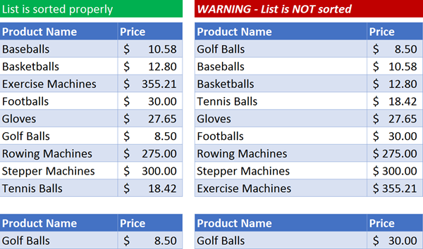
Excel has the ability to sort data in a variety of ways:
- Alphabetically
- Numerically
- Chronologically
In addition, the data can be sorted in either ascending (smallest to largest) or descending (largest to smallest) order.
Sorted lists are useful when printing or for scanning when looking for information. It is far easier to locate an item in a sorted list than if the list was seemingly random. Imagine trying to find a person’s name in a list that has been sorted by employee number. Assuming your company doesn’t hire people in alphabetical order, this will prove difficult.
Sorted lists will dramatically improve search times in functions like VLOOKUP (see previous post “Supercharge Your VLOOKUP Functions in Excel”.) The risk is that if a user were to sort a list being scanned by a VLOOKUP, and the VLOOKUP was NOT utilizing “exact matching” logic, incorrect information can easily be returned. If we trust our formulas to work properly, we may not realize we have been given erroneous data.
If you want to keep tabs on the sort order of a list, we can do this with an extremely simple formula and a few tricks to spice up the visuals. Our solution will utilize four key Excel features:
- Array Functions
- Conditional Logic (optional)
- Conditional Formatting (optional)
- Custom Number Formatting (optional)
It sounds like it’s going to be a lot of work, but once you see it working, it’s actually quite easy and quick to implement. Some of the above mentioned features are not necessary to solve the immediate problem of being alerted to an unsorted list, but they are included so you can add a few more tricks to your Excel toolbox.
Example of Things Going Wrong
Consider the below list:
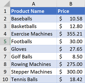
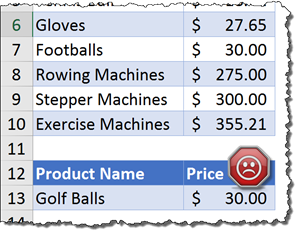
If we were to use this list in a VLOOKUP, and we were not using “exact match” logic, we would have to ensure that the list were never to be sorted by any column other than the Product Name column.
Example: Cell B13 contains a VLOOKUP function that takes the user input from cell A13, finds the item in the Product Name column, and then returns a price from the Price column of the list.
=VLOOKUP(A13,A2:A10,2)
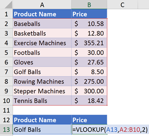
This VLOOKUP is not using “exact match” logic, but since the list is sorted by Product Name, the returned Price is correct (and super fast).
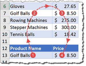
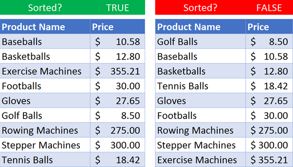
Suppose someone were to sort the list so the items were listed in ascending order by Price? Would the VLOOKUP function’s answer be correct? The answer is a “No”.
What we want is to be alerted for when this list changes from “sorted ascending by product” to any other sort order.
Step 1 – Determine the Sort Status
We will check the sort order of the Product Name column by writing the following array formula.
CAUTION: If you have never created an array formula, you MUST enter the formula with a CTRL-SHIFT-ENTER key combination. A traditional ENTER key will not build the formula properly.
{=AND((A2:A9)<=(A3:A10))} (do not type the beginning and ending braces; they will be created when you press the CTRL-SHIFT-ENTER key combination.)
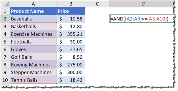
So what exactly is this formula doing? It’s actually quite simple, and that’s where the elegance lies.
The formula takes a list of products from A2:A9 and compares it to a list of products from A3:A10.
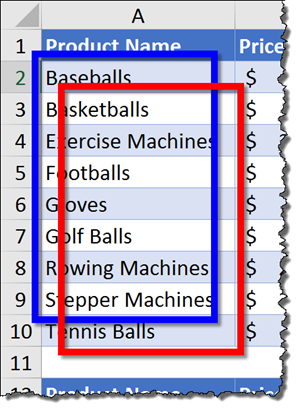
The formula checks to see if each item in the first list is less than or equal to the corresponding item in the second list. Because this was constructed as an array function, the actual process looks something like this:
A2<=A3
A3<=A4
A4<=A5
A5<=A6
etc…
The list of results would appear as follows:
True
True
True
True
etc…
Because we are placing all of the results under the control of an AND function, if all of the individual tests result in TRUE, the entire test is true and is therefore a sorted list. If even one test were to result in a FALSE response, the entire test would fail resulting in a final FALSE answer.
You COULD stop right here and go home, satisfied with a job well done… but let’s jazz it up a bit.
Step 2 – Conditional Logic to Display a Status Message
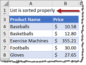
If you want to have message displaying the status of the list’s sort order, you could write an IF formula like the following: (Remember – it’s an ARRAY formula)
{=IF(AND((A4:A11)<=(A5:A12)),”List is sorted properly”,”WARNING – List is NOT sorted”)}
Step 3 – Use Conditional Formatting to Apply Fill Color to Message
There are a variety of ways you could apply conditional formatting to the message.
- If A1 is equal to “List is sorted properly” then fill color equals green
- If A1 is equal to “WARNING – List is not sorted” then fill color equals red
Just to have a bit more fun, and learn a few more tricks, let’s do it a bit differently.
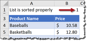
We have entered the array formula for the IF messages in cell A1. Let’s enter the below formula in cell B1.
{=IF(AND((A4:A11)<=(A5:A12)),1,0)}
This will return a “1” if the list is sorted and a “0” if the list is unsorted. We will treat the “1” as “True” and the “0” as “False”.
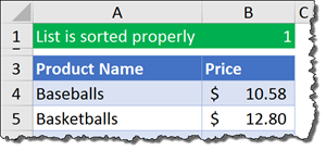
Select cells A1:B1 and color the cells using a white font color with a green fill color. This will serve as the default “all is well” color scheme.
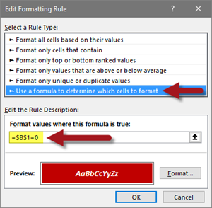
Using Conditional Formatting, select cells A1:B1 and create a new rule using a formula to format the cells. Enter the formula below and set your colors accordingly (such as bold, white text on a dark red background.)
=$B$1=0
Conditional Formatting colors always supersede manually applied colors. For more information on how colors are applied in Excel, see the post “Excel Color – Order of Application (Hierarchy)”.

Step 4 – Making Data Invisible Using a Custom Number Format
The final trick is to hide the “1” or “0” displayed in cell B1. You could set the font color to match the fill color, but if the fill color changes, the number will reveal itself.
Select cell B1 and open the Format Cells dialog box. On the Number tab, select the Custom category on the left and enter three semi-colons in the Type: field.
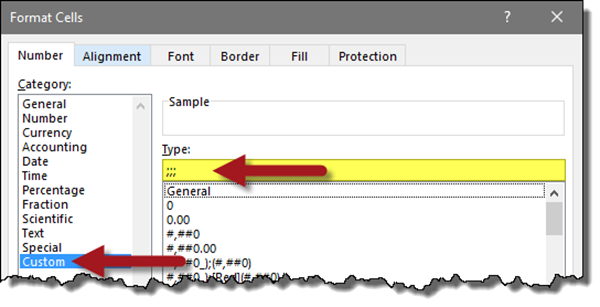
If you are not familiar with custom number formatting, codes are broken into four presentation categories:
How we display
- positive numbers
- negative numbers
- zeroes
- text
Each set of codes is separated by a semi-colon. By typing the semi-colons WITHOUT any codes, we are saying “don’t display ANYTHING”. This will make anything typed into a cell invisible, regardless of font color or fill color settings.
