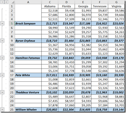
Suppose you have data stored in multiple locations but you wish to create a chart from all of the data sources as if they were stored as a single data source. You could spend time manually copying and pasting the data into a single, unified list, but this may prove difficult if the data is stored in a non-tabular structure such as a cross-table.
Take the following three cross-tables:
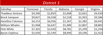
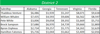
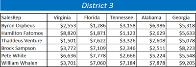
The objective is to consolidate all of the sales reps sales for each of the five states. The problem is we cannot simply create a 3D SUM function (i.e. =SUM(‘District1:District3’!B4)) that collects all of the numbers from each of the same cell addresses from each sheet. Notice how none of the sales reps are on the same row and none of the states are in the same columns. We would have to manually scan each cell and target them separately for each sales rep and state. Luckily, Excel has a tool that can figure this our for us in no time flat.
Consolidate
Excel’s Consolidate tool allows us to point to a variety of data sets and then aggregate them together into a single summary set based on an aggregation method of our choosing. We can consolidate the lists in one of two ways:
- Consolidate by Position
When the data in the source areas is arranged in the same order and uses the same labels. Use this method to consolidate data from a series of worksheets, such as departmental budget worksheets that have been created from the same template.
- Consolidate by Category
When the data in the source areas is not arranged in the same order but uses the same labels. Use this method to consolidate data from a series of worksheets that have different layouts but have the same data labels.
NOTE: Consolidating data by category is similar to creating a PivotTable. With a PivotTable, however, you can easily reorganize the categories. If you want a more flexible consolidation by category, consider creating a PivotTable instead.
The process for consolidation is similar for either of these scenarios.
Selecting the Data for Consolidation
With your cursor resting on the sheet that will contain the consolidated data (most likely a new empty sheet), select Data (Ribbon) –> Data Tools (Group) –> Consolidate.

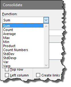
This will launch the Consolidate dialog box. Select the method of aggregation from the Function dropdown list (i.e. SUM).
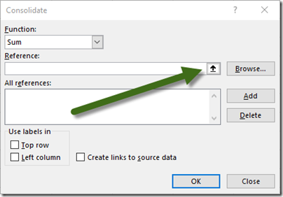
In the Reference section, select the ![]() button to browse to the data and highlight the desired cells.
button to browse to the data and highlight the desired cells.
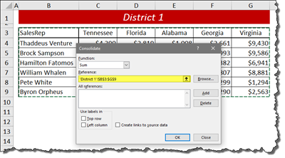
If you are consolidating by position, select the DATA ONLY (no headings). If you are consolidating by category, select the data and the related row and column headings. In the example below, we are selecting data by category.
Click the ![]() button to add the selected range to the All References… list.
button to add the selected range to the All References… list.
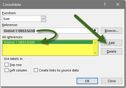
Repeat this process for all of the remaining data ranges.
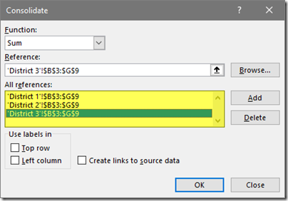
Step 2 – Setting Consolidation Options and Linking
If your data has headings across the top of the columns, and you wish for Excel to aggregate based on those headings, select ![]() .
.
If your data has headings down the left side of the data, and you wish for Excel to aggregate based on those headings, select ![]() .
.
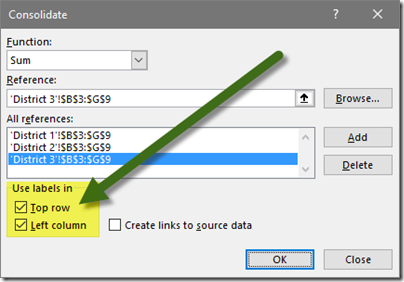
If you are consolidating data by similar cell addresses, leave these two options unchecked.
If you want the data in the consolidated report to update when the original source data changes, select ![]() .
.
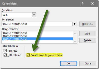
Click OK to view the results of the consolidation.
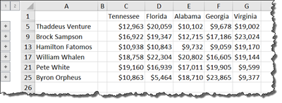
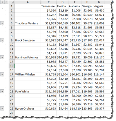
Because this example used the data’s row and column headings, the data was aggregated correctly based on sales rep name and state name regardless of the location of said data within each of the tables.
In addition, the aggregated data utilizes an outline structure that allows us to “drill down” into each of the sales reps totals to see what values make up the totals. This is because we checked the box labeled ![]() .
.
Extra Credit #1 – Charting the Consolidated Data
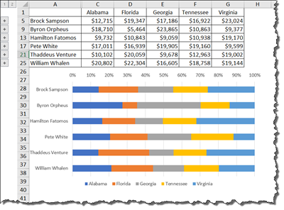
Now that you have consolidated all of the like rows and like columns together into a summary report, you can now make loads and loads of wonderful charts and graphs.
Extra Credit #2 – Making the Consolidated Data Look Pretty
When you have dozens or hundreds of rows of data between each total row, it can become difficult to zero-in on the total rows. A nice touch to the expanded summary report would be to highlight the total rows for each sales rep. We don’t want to do this manually because it could require hundreds (or thousands) of manual highlights, and the data may change structure over time. A creative way to accomplish this is to utilize Conditional Formatting.
Step 1 – Select the Data
Highlight all of the data. It is important that you begin your highlight from what would be the upper-left hand corner of the data. This is necessary for the conditional formatting logic to “spread” through the remainder of the data. In this example, we are beginning the highlight in cell A1.
Step 2 – Create a Conditional Formatting Rule
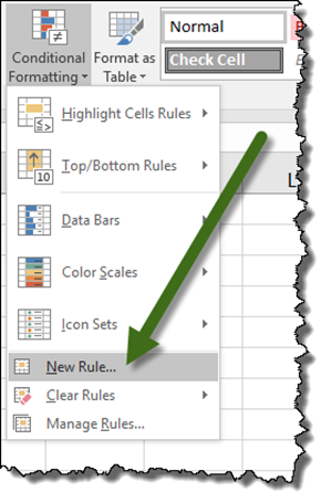
Select Home (Ribbon) –> Styles (Group) –> Conditional Formatting –> New Rule…
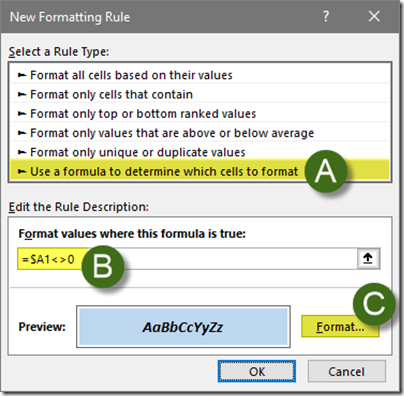
(A) In the New Formatting Rule dialog box, select Use a formula to determine which cells to format.
(B) In the Rule Description, enter the following rule: =$A1<>0
The logic of this formula is to have each cell examine its own column “A” cell to see if the cell is not equal to zero. All of the cells in column “A” are valued as zero except for those with names.
(C) Format the summary rows to a font and cell color of your choosing.
The data will now be displayed with easy to locate total rows.
